Turbulence and Convection

Mixing of the atmosphere

Learning Objectives

Understand what ‘turbulence’ is.
Describe what causes a flow to be turbulent.
Explain how can we quantify the degree of turbulence.
Understand how this small scale randomness can impact larger scale processes.
Explain how we can describe / model convective transport.

Class Conduct

Talking during class can disrupt the learning experience of your classmates.

It is okay to quietly ask your neighbors questions or discuss issues relating to class content
It is not okay to have loud/long conversations

Class Conduct (iClicker)

Talking during class can disrupt the learning experience of your classmates.

True
False

Energy Transfer

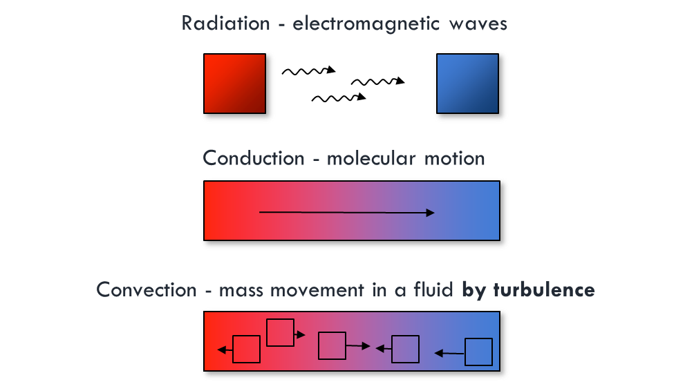
Laminar vs. Turbulent Flow

Laminar flow: parallel streamlines

Mixing is inefficient, only occurs by diffusion

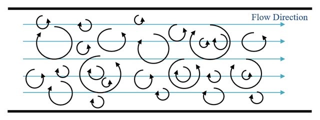
Turbulent flow: irregular streamlines

Mixing is very efficient and occurs mainly by convection

Turbulence

Turbulence is a feature of flows, not fluids.

Turbulent flows are very efficient in equalizing temperature and concentration gradients:
- In the Atmosphere, turbulent flows are 10⁵ times more efficient than molecular diffusion

Eddies

Coherent parts within the flow which have the same properties.

Eddies exist in a wide range of different sizes
- “Big whorls have little whorls which feed on their velocity, and little whorls have lesser whorls, and so on to viscosity.”
  - Richardson, 1922

Eddies

Coherent parts within the flow which have the same properties.

Eddies exist in a wide range of different sizes
The smallest eddies dissipate to heat

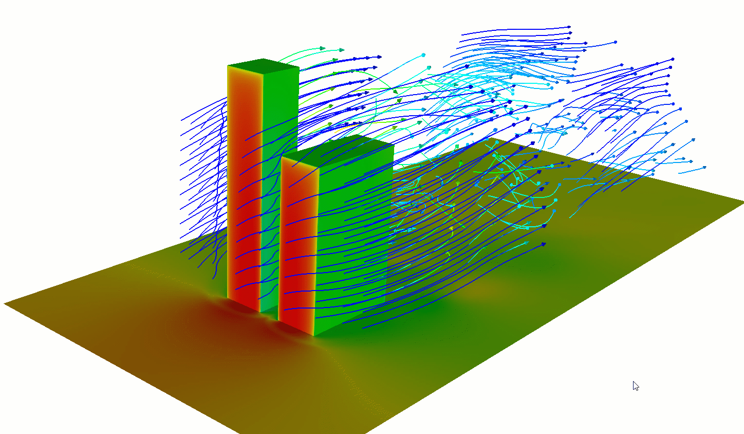
Forced (Mechanical) Convection

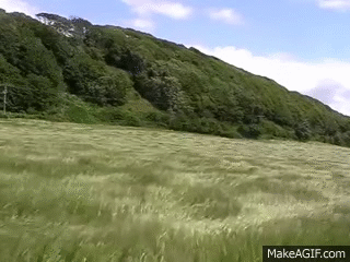
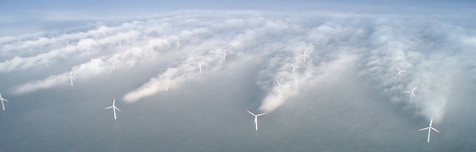
Wind moving past obstacles (trees, buildings, etc.) creates eddies mechanically by disturbing flow.

Eddy size related to the size of the obstacle and flow velocity

Forced (Mechanical) Convection

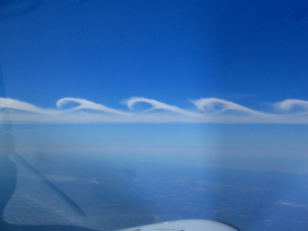
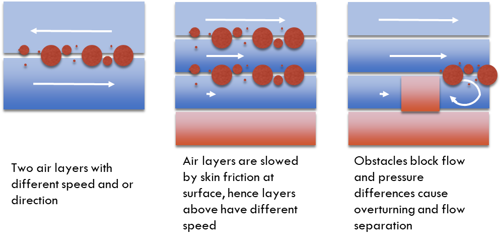
Air moving at different speeds, or in different directions, creates shear stress.

Causes turbulence and eddies
Explains the turbulence you feel in an airplane

Forced (Mechanical) Convection

Wind moving over a natural surface experiences skin friction as it drags along

Greater over rough surfaces

Forced (Mechanical) Convection

Requires a continual supply of kinetic energy from the flow. It comes from the mean wind speed.

Wind is driven by pressure/temperature gradients at larger scales (we’ll discuss this later)

Forced (Mechanical) Convection

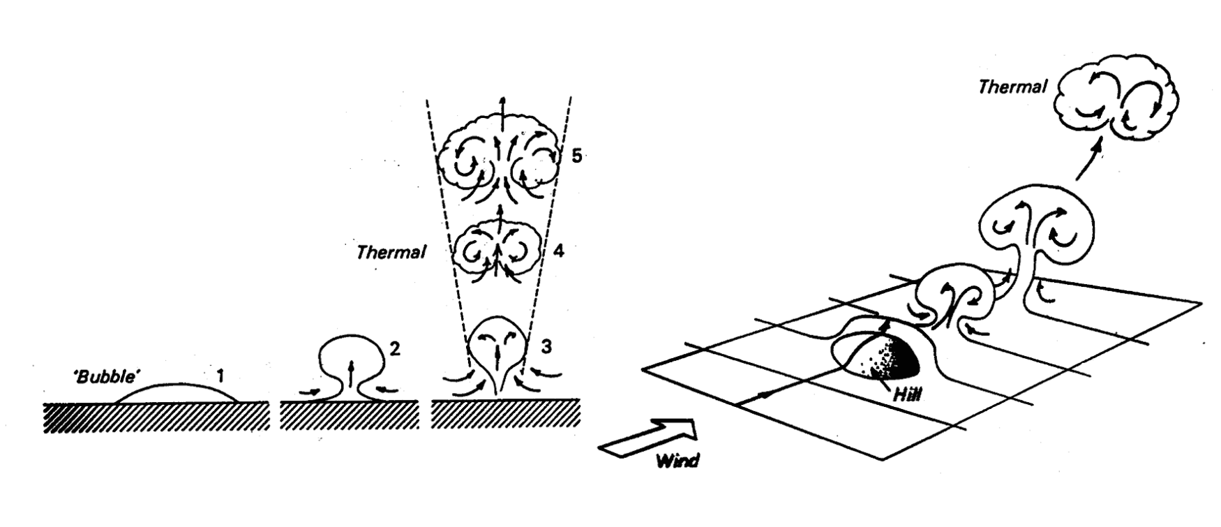
We can have three different scenarios that create turbulence mechanically

Free (Thermal) Convection

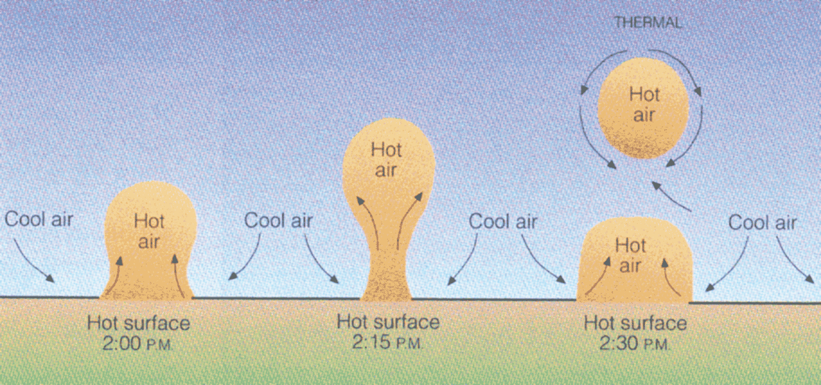
Surface heating differences → density differences → buoyancy differences → convection.

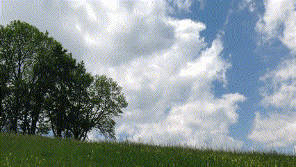
Free (Thermal) Convection

Buoyant parcels are often semi-organized into ‘plumes’; rising thermals form convection cells.

T.R. Oke (1987)

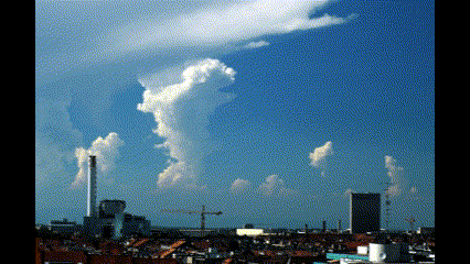
Free (Thermal) Convection

Intense Convection > Thunderstorm

Turbulence (iClicker)

Which of the following characteristics is not applicable to a turbulent flow?

A Mixing is very efficient
B Flow is highly irregular with 3D curved streamlines
C Exchange only occurs by molecular diffusion
D A range of eddies of different scale exist
E Produced by mechanical and/or thermal processes

Eddy Size and Source of Convection

Day: wide range of eddy sizes
- Free convection (heating)
- Forced convection (wind)
Night: Eddies are small
- Forced (wind)

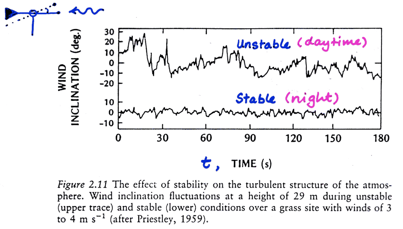
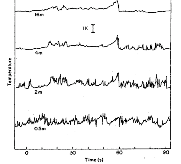
Traces of vertical wind near the same surface with same wind speed with and without surface heating.

Turbulence & Air Temperatures

Nearest the ground with both small and large eddies
At greater heights only the buoyant plumes remain (large eddies).
- The intermittent convection ‘plumes’ can be traced as they move upward

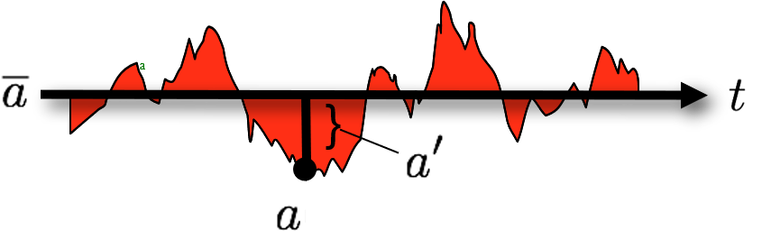
Reynolds Decomposition

Turbulent properties appear chaotic, but can be analyzed by deconstructing them into two parts:

The time mean (e.g., \(\bar{a}\))
The instantaneous deviation from the mean (e.g., \(a^{\prime}\))

This is called Reynolds’ decomposition

\[ a = \bar{a} + a^{\prime} \qquad(1)\]

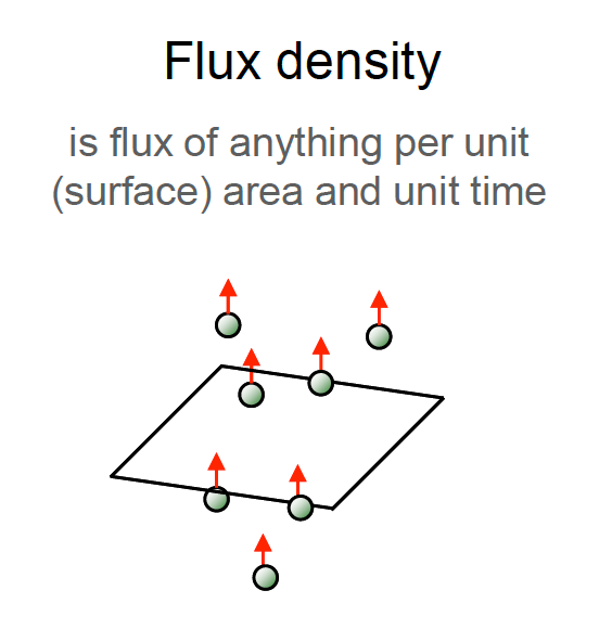
Convective transport

Eddies in a turbulent flow fulfill the same role as molecules do in molecular diffusion.

Convection transports heat, mass and momentum as the eddies ‘jump’ up and down.

Flux Gradient Method

For sensible heat flux we can write:

\[ H_s = -K C_a \frac{T_2 - T_1}{z_2 - z_1} \qquad(2)\]

\(K\) is the eddy diffusivity (m² s^-1) and \(C_a\) is the heat capacity of dry air
Note the similarity to Fouriers Law!

Eddy Diffusivity

\(K\) varies as a function of the intensity of the turbulence and therefore varies

Wind speed > \(K\) will increase as a function of wind speed
Stability > \(K\) is greater for unstable conditions
Surface roughness
- All else equal \(K\) will be higher for a rougher surface
  - \(K_{forest} > K_{water}\)

Flux Gradient Method

Similar equations can be written for the fluxes of H₂O, CO₂, etc.

\[ F = -K C^* \frac{f_2 - f_1}{z_2 - z_1} \qquad(3)\]

Here; \(F\) is the flux of some property (\(f\)), and \(C^*\) is a “unit conversion constant”
Note: Equation 3 is for example only, you won’t be asked to evaluate it
- You will be asked to evaluate Equation 2

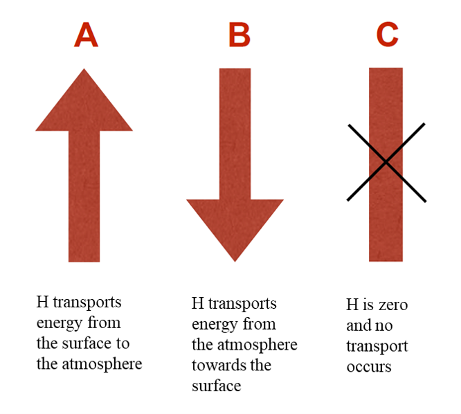
Measuring Sensible Heat Flux

Test your knowledge

What is the direction of the sensible heat flux density \(H_s\)?

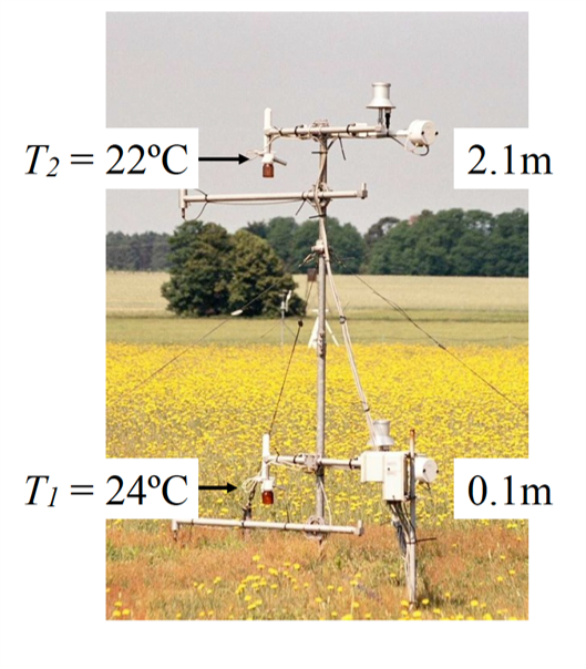
Example Calculation

Assume \(K\) = 0.25 m² s^-1 and \(C_a\) = 1200 J m^-3 K^-1, what is H?

\(H_S = -K C_a \frac{T_2 - T_1}{z_2 - z_1}\)

A 300 W m^-2
B -300 W m^-2
C 600 W m^-2
D 150 W m^-2
E -150 W m^-2

Example Calculation

Assume \(K\) = 0.25 m² s^-1 and \(C_a\) = 1200 J m^-3 K^-1, what is \(H_S\)?

\(H_S = -K C_a \frac{T_2 - T_1}{z_2 - z_1}\)

T1 = 24 #C
T2 = 22 #C
z1 = 0.1 #C
z2 = 2.1 #C
K = 0.25 #m2 s-1
C_a = 1200 #J m-3 K-1
H = -K*C_a*(T2-T1)/(z2-z1)

A 300 W m^-2

Stable vs Unstable

In which condition do you think K is generally higher?

A Stable
B Unstable

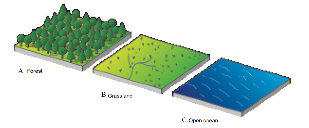
Effect of Surface Roughness

Assume high wind speed and little heating. Which landscape do you think has the highest \(K\) (at 20m above ground)?

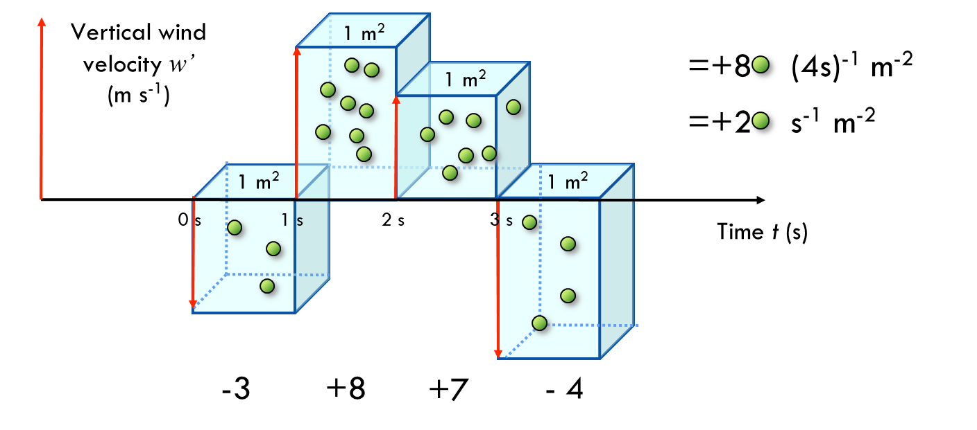
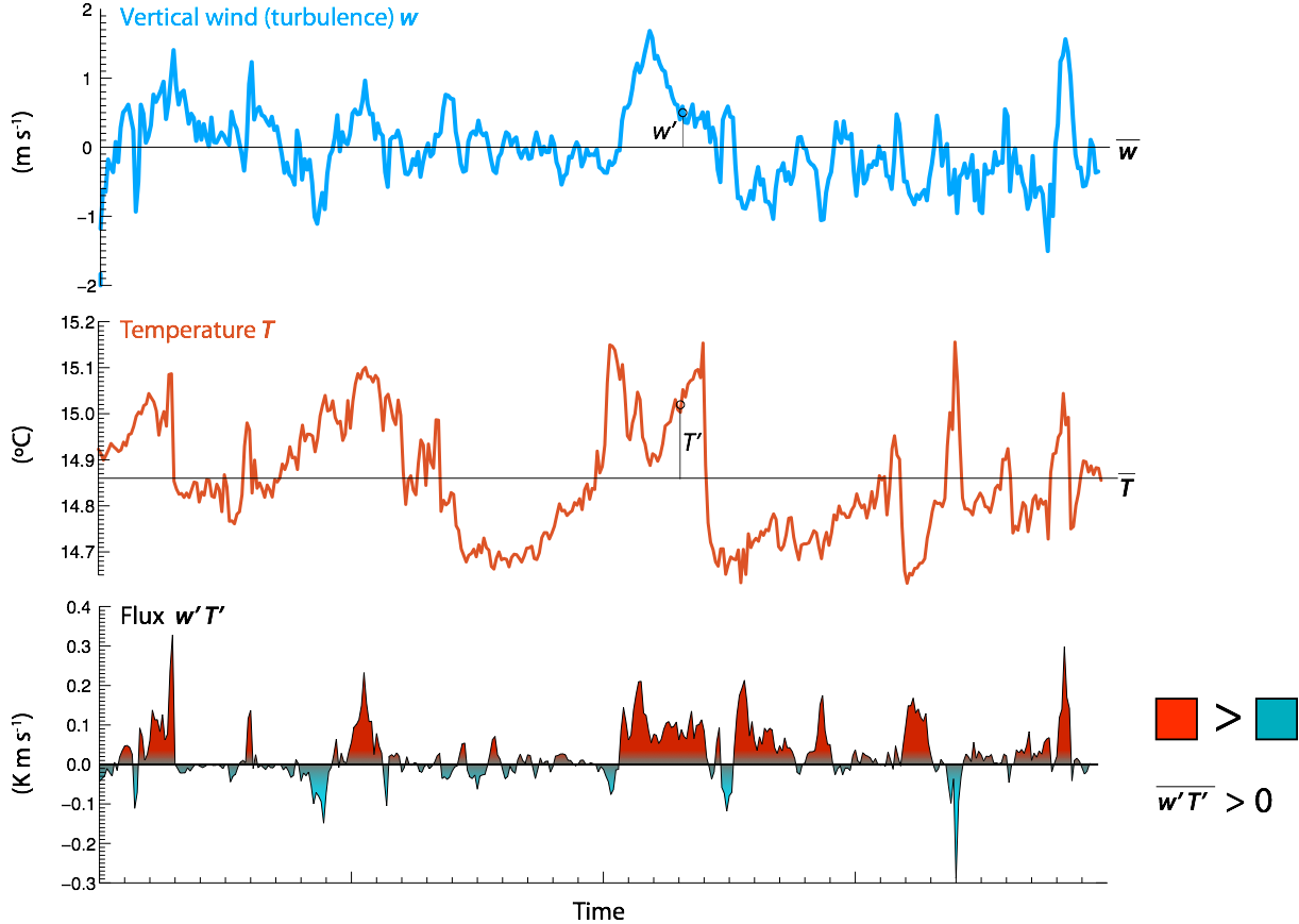
Convective Transport

Transport is accomplished because each eddy has a vertical velocity (\(w\)) and a concentrations (\(c\))
- \(w\) wets the rate and direction of transport of various atmospheric properties (\(T\), \(\rho_v\), etc.)

Convective Transport

The instantaneous flux density is the product of \(w^{\prime}\) and \(c^{\prime}\).

The average flux density is found by counting all the instantaneous products (w’ and c’) summing them, and averaging over the time period:

Reynolds Notation

A flux density is the average of all the instantaneous products of the vertical speeds of the eddies and the properties they carry:

\[ F_c = \bar{w^{\prime}c^{\prime}} \qquad(4)\]

\(w^{\prime}\) and \(c^{\prime}\) are the instantaneous vertical wind velocity and concentration of an entity
- The concentrations must be measured within about 30 cm of where w is measured
These multiplications must be made typically 20 times each second and averaged over larger time intervals (usually 30 minutes).
- This means we must do 36,000 multiplications per 30 minutes!

Eddy Covariance Method

This is called the eddy covariance method because the expression on the right Equation 4 is called the covariance of \(w^{\prime}\) and \(c^{\prime}\)

For the case of sensible heat flux density we write:

\[ F_c = C_a \bar{w^{\prime}c^{\prime}} \qquad(5)\]

Where \(C_a\) is the heat capacity of air (1200 J m^-3 K^-1)

Eddy Covariance Systems

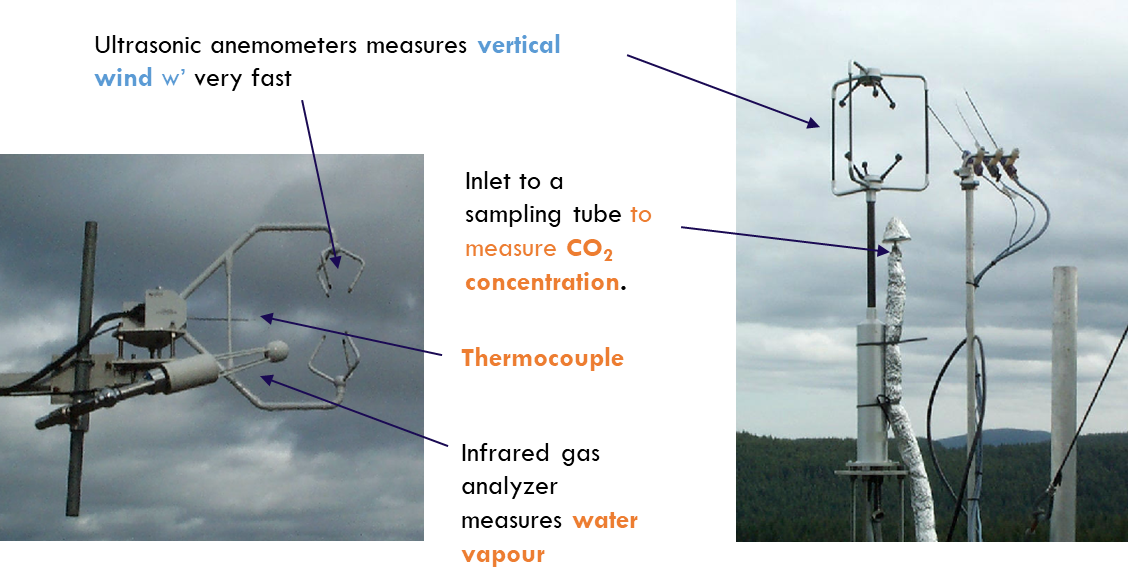
Example - Sensible heat flux density

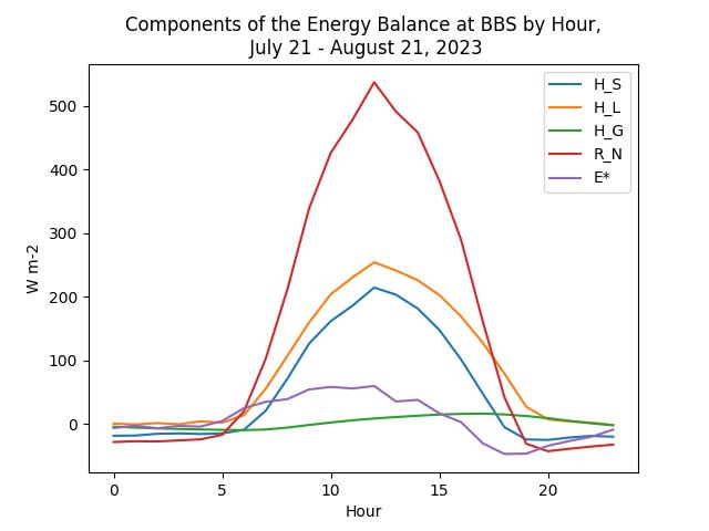
Latent Heat Flux Density

For many ecosystems, with a sufficient moisture supply latent heat flux \(H_L\) will exceed sensible heat flux \(H_S\).

:::{column width=“50%”}

\(H_L\) is equivalent evapotranspiration from the ecosystem (when \(H_L > 0\) W m^-2):
- Evaporation (from surfaces) + transpiration (from plants)

:::{column width=“50%”}

::: ::::

Take home points

Measurement of convective exchange is more difficult compared to conduction / diffusion.
Fluid flow can be laminar or turbulent.
Eddies are coherent parts of the flow that show homogeneous properties.
Mechanical and thermal convection create eddies (turbulence).
We can use Reynold’s notation to separate a signal into a turbulent and a mean part.
Direct measurement using eddy covariance method is possible - but requires sophisticated and expensive instrumentation and more tedious data analysis.