Lab 2: Radiation

This assignment is worth 15 points.

Objectives

This lab will have two components.

Measure the coefficient of reflection for a variety of natural surfaces and calculate coefficients of absorption and transmission
Describe how coefficients of absorption, reflection and transmission differ between visible and near-infrared light sources
Describe how properties of natural surfaces affect coefficients of absorption, reflection and transmission of radiation
Define the term albedo
- Calculate the flux density of solar radiation leaving the Sun’s surface and reaching the Earth’s surface
- Define terms used in Earth’s radiation budget
Define the Stefan-Boltzman Law

Table 1: Definitions for symbols/abbreviations and constants used in this lab.
Symbol	Name	Definition
\(T\)	Temperature	Quantitatification of the heat present in an object (in K unless specified otherwise)
\(\lambda\)	Wavelength	The distance between the crest of of two waves (of elector magnetic radiation).
\(SW\)	Short wave radiation	Electromagnetic radiation with \(\lambda\) less than and 3 \(\mu m\). Includes ultraviolet; visible; and near-infrared radiation.
\(LW\)	Long wave radiation	Electromagnetic radiation with \(\lambda\) greater than 3 \(\mu m\). Includes thermal radiation (sensible heat).
\(R_n\)	Net Radiation	The sum of all incoming (\(\downarrow\)) and outgoing (\(\uparrow\)) radiation (both \(SW\) and \(LW\)).
\(a\)	Absorptivity	Radiation that is absorbed by an object; adding energy to the object and increasing its temperature.
\(\tau\)	Transitivity	Radiation that passes through an object.
\(\alpha\)	Reflectivity	Radiation that is reflected by a object.
\(E_b\)	Black-body emissivity	An idealized estimate of radiative flux density based on an object’s temperature assuming its a black-body see Equation 2
\(\sigma_b\)	Stefan-Boltzman constant	5.67 x 10 \(^{-8}\) W m\(^{-2}\) K\(^{-4}\)
\(I_o\)	Solar constant	1361\(W m^{-2}\)

1 Theory

This part of the lab is designed to acquaint you with the component fluxes of a radiation budget.

Short-wave vs. Long-wave Radiation

In meteorology, we broadly classify radiation by wavelength \(\lambda\) as either short-wave (\(SW\)) or long-wave (\(LW\)). Units of wavelength are often given in micrometers (1 \(\mu m\) = 10^-6 m). The distinction is relative and you may see variability across the literature. We will define them as:

Short-wave (\(SW\)): \(\lambda < 3 \mu m\)
Long-wave (\(LW\)): \(\lambda >= 3 \mu m\)

Radiation Balance

Recall from lecture^{1 2 3}: radiation may interact with an object in one of three ways; it can be absorbed, transmitted, or reflected.

\[ a_\lambda + \tau_\lambda + \alpha_\lambda = 1 \tag{1}\]

The coefficients of absorption (\(a_\lambda\)), transmission (\(\tau_\lambda\)), and reflection (\(\alpha_\lambda\)) vary depending on the wavelength \(\lambda\) of the incident radiation and the properties of the object.
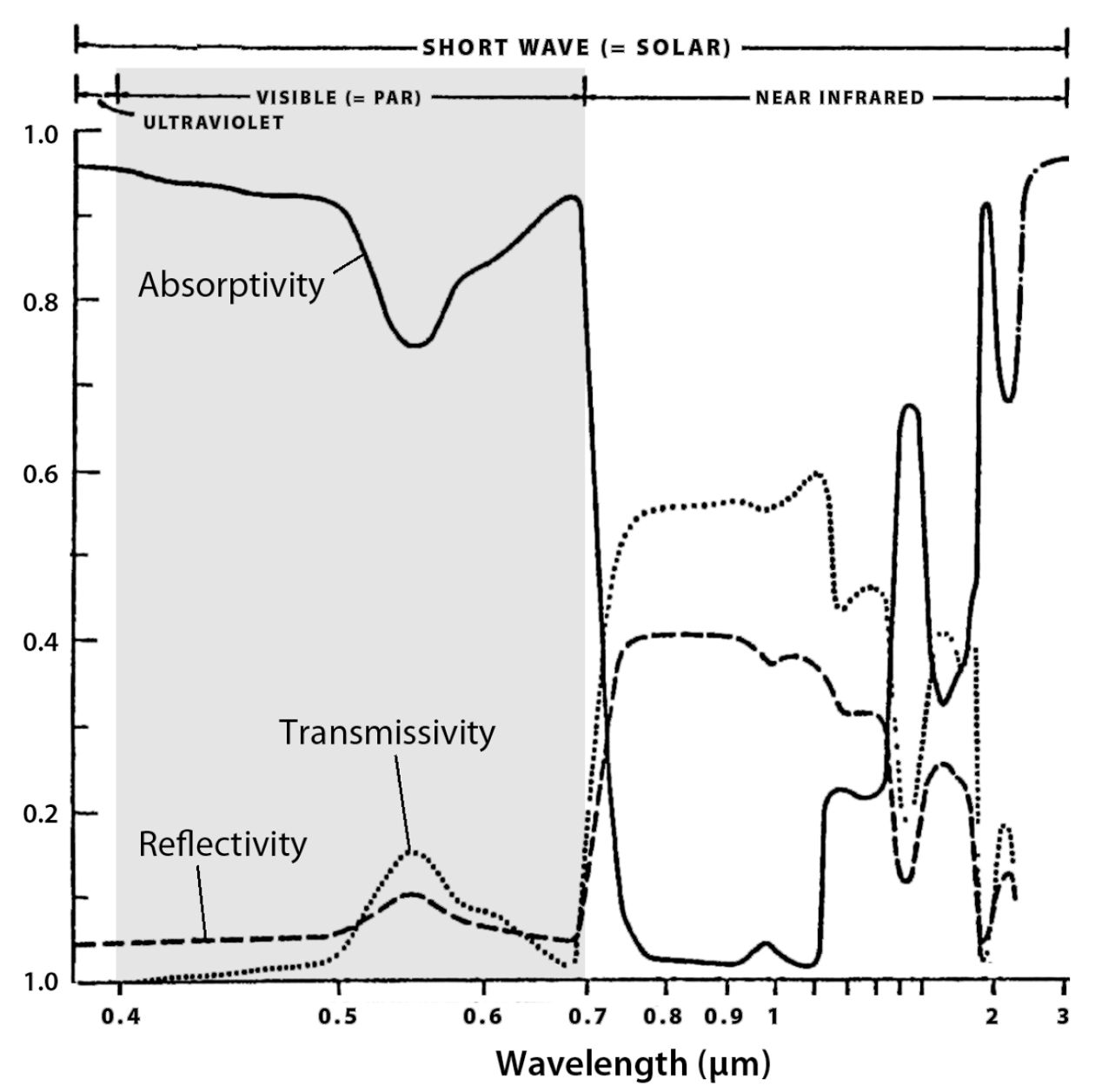
Plant leaves have interesting radiative properties that are part of the plants’ adaptation to their environments. The coefficients of reflection, transmission and absorption are strongly dependent on wavelength as shown by a typical example in Figure 1.
- Energy is strongly absorbed in the visible region where radiation is active in photosynthesis.
- In the near infrared region (NIR) radiation is more strongly reflected and transmitted.

Figure 1: Spectral absorptivity, reflectivity and transmissivity of a poplar leaf

Radiative Output of the Sun

RECALL:

Flux	Flux Density
Energy flow, Watts or W [i.e., Joules per second]	Energy flow divided by area (W m^-2).

Recall from lecture¹; the radiative output of an object is proportional to its temperature. The radiative flux density can be approximated (for an idealized object) using the Stefan-Boltzman Law for a “Black Body”:

\[ E_b = \sigma_b T^4 \tag{2}\]

However, in reality, we must adjust the calculation to account for the emissivity coefficient (\(\epsilon\)) of the object. The \(\epsilon\) value represents the actual radiative output of a real object relative to the emission of an idealized Black-body at the same temperature. To do to this we can adjust and use the Stefan-Boltzman Law for a “Grey Body”:

\[ E_g = \epsilon\sigma_b T^4 \tag{3}\]

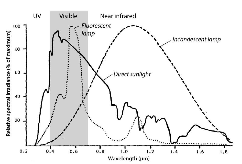
To describe a radiation source, we can plot its spectrum. Spectra for solar radiation and radiation from a fluorescent lamp and an incandescent tungsten filament lamp are shown in Figure 2.

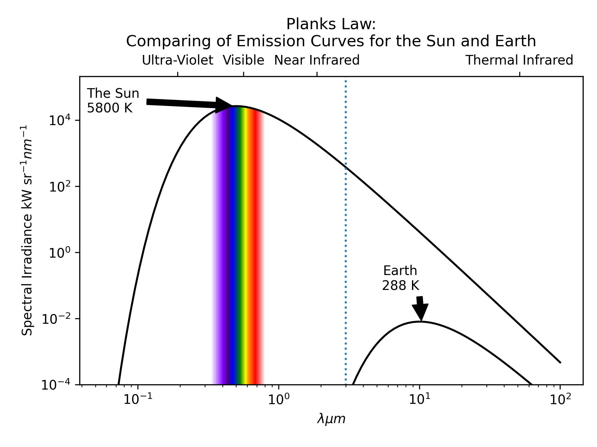
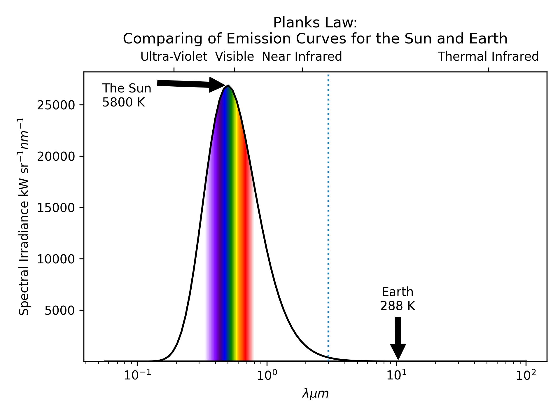
Because the sun is very hot (\(\approx\) 5800 K) it emits a large amount of radiation across a wide range of the wavelengths Figure 3.
- It is important to note that: short-wave radiation makes up the overwhelming majority (99+%) of the sun’s radiative output
Because the earth is relatively cool (\(\approx\) 288 K) it emits a smaller amount of radiation across a narrower range of wavelengths.
- It is important to note that: the earth does not emit short-wave radiation because it is to cool.

Figure 2: Observed spectral irradiance of sunlight, a Tungsten incandescent land (2700°C) and a fluorescent lamp. In this diagram, the spectra have been adjusted to equal peak heights.

(a) Black-body spectral irradiance of the Sun and Earth (logarithmic scale).

Radiation Reaching the Earth

Thankfully, on Earth, we are not subject to the full radiative output of the sun. The solar beam spreads out (dissipates) on the (approximately) 150 million km journey from the sun to the Earth. Satellite measurements indicate that the mean radiative flux density a the top of the atmosphere is 1361 W m^-2; this value is known as the solar constant \(I_0\). Knowing the value of the solar constant, we can do some calculations to deduce the total radiative flux of the sun in W. The calculation is shown in the example below in Example 1 using R code. See the output at the bottom for the approximate value. Note: This is just an illustrative example to expose you to programmatic calculations using R. You do not need to know/learn R for this course.

The earth has a slightly eccentric orbit - it is elliptical (slightly oval shaped) and off center. This means that the distance between the earth and the sun vary slightly. The Earth is closest to the sun (147 million km) on the perihelion which occurs in early January and it is farthest from the sun (152 million km) on the aphelion in early July Figure 4 (a). Consequently, the true flux density of the solar beam at the top of Earth’s atmosphere will deviate slightly from the solar constant over the course of the year.

Example 1

# Deriving solar radiative output from the solar constant.
# Defining our variables
Solar_Constant = 1361

# Note - when writing code, we can use the "e" character as shorthand for scientific notation
# 1.5e11 = 1.5 x 10^11
Radius_of_Orbit = 1.5e11

# Calculate the total area over which the solar beam is spread at the average distance between the earth and the sun
# Area = 4πr2
Area = 4*pi*Radius_of_Orbit**2

# To convert the flux density (Solar_Constant) to a total Flux we multiply by area
Solar_Flux = Solar_Constant*Area

# This function formats a text (string) output the "%s" values are replaced with the variable(s) listed after the string
Output <- sprintf('Radiative Output (Flux) of the sun %s W',Solar_Flux)

# This function prints us a cleanly formatted output
writeLines(Output)

Radiative Output (Flux) of the sun 3.84813684138214e+26 W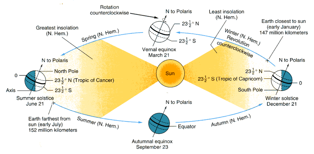

(a) Simplified diagram showing the seasonal changes in the Sun-Earth geometry.

Balancing the Budget

Following equation Equation 1. A portion of incoming short-wave radiation (\(SW \downarrow\)) that hits Earth is reflected by the surface back towards the sky as outgoing short-wave radiation (\(SW \uparrow\)). We can define the term albedo to describe reflected short wave radiation (\(\alpha_SW\)):

\[ albedo = \alpha_{SW} = \frac{\uparrow SW}{\downarrow SW} \tag{4}\]

Following Equation 1, the earth can also absorb shortwave radiation (\(a_{SW}\)). The earth (as a whole) also does not transmit short-wave radiation (\(\tau_{SW}\)). However objects on or near its surface, such as leaves can Figure 1. When dealing with an opaque object such as a the surface of the earth, we can define absorption as Equation 5, but when dealing with transparent objects such as leaves or water, we must define absorption as Equation 6:

\[ a_{\lambda} = 1 - \alpha_{\lambda} \tag{5}\]

\[ a_{\lambda} = 1 - \alpha_{\lambda} - \tau_{\lambda} \tag{6}\]

Note Equation 1 and Equation 6 are equivalent to one another.
Note you can calculate \(\tau\) using the same approach as in Equation 4, you would just use transmitted \(SW\) in the numerator instead of reflected \(SW\)

Following Equation 5, any short-wave radiation that is not reelected by the Earth’s surface, will be absorbed. When short-wave radiation is absorbed, the energy is “transformed” from one form to another. Some of the energy goes towards phase changes of water, some of it goes into chemical reactions (e.g., photosynthesis), and a large portion of it is re-emitted as outgoing long-wave radiation (\(LW\uparrow\)), aka. thermal radiation. Following

Combining these Net All-Wave Radiation (\(R_n\)), as defined in Equation 7, is the sum of all incoming (\(\downarrow\)) and outgoing (\(\uparrow\)) short-wave (\(SW\)) and long-wave (\(LW\)) radiation. Net radiation can tell us how much energy is entering (positive) or leaving (negative) the site at any given time. If net \((R_n)\) is a large positive number, that indicates significant energy input, which would cause the land surface at the site to warm up. Conversely, if \((R_n)\) is negative, that means the site is loosing energy (cooling off).

\[ R_n = (SW \downarrow - SW \uparrow) + (LW \downarrow - LW \uparrow) \tag{7}\]

The all-wave budget could also be considered to consist of a net short-wave budget, \(SW^* = SW\downarrow - SW\uparrow\) and a long-wave budget \(LW^* = LW\downarrow - LW\uparrow\) , i.e. \(R_n = SW^* + LW^*\). The sign convention adopted here is that individual fluxes have no sign (i.e., always positive) but net fluxes (those with an asterisk) are positive if they are a net energy gain for the surface, and negative if they are a net energy loss.

Questions

The following simple computations help to demonstrate the radiation relationships existing between the Sun (the Earth’s only source of energy) and the Earth and the Earth and Space. They explain the sizes of the radiation streams between these bodies and so doing illustrate the concept of a radiation budget.

Question 1 [1 points]

Use the Stefan-Botzman Law for a Black-Body (Equation 2) to estimate the radiative flux density of the sun, which has a surface temperature of approximately 5800 K.

Answer:

T = 5800
sigma_b = 5.67e-8

E_b = sigma_b*T**4

sprintf('%s W m-2',E_b)

[1] "64164532.32 W m-2"

Question 2 [2 points]

The radiative flux of the Sun is approximately 3.85 ×10²⁶ W (see Example 1). Given the Sun’s radius to be 6.96 × 10⁸ m, find the average flux density in W m^-2 of solar (short-wave) radiation leaving the Sun’s surface. Hint: The area of a sphere: A=4πr2
Why is this number lower than what you got using the Equation 2?

Flux = 3.85e26
Radius = 6.96e8

# To get density:

# First we need to calculate the area of the sphere
# Area = 4πr2

Area = 4*pi*Radius**2

# Then divide flux by area

Flux_Density = Flux/Area

sprintf('%s W m-2',Flux_Density)

[1] "63245901.3434524 W m-2"

It is lower - the sun isn’t a black body so it isn’t an perfect emitter. To get a better estimate you can adjust the Botlzman equation to account for emissivity \(\epsilon\)

Question 3 [0.5 points]

Following these calculations - what would the approximate emissivity (\(\epsilon\)) of the sun be?

Emissivity = Flux_Density/E_b
print(Emissivity)

[1] 0.9856832

Question 4 [1 points]

The value of the solar constant \(I_0\) is for the Earth’s mean distance from the sun. How would the distnace between the earth and the sun differ over the year? What would the approximate difference in radiate flux density at the top of the atmosphere be between the perihelion and aphelion respectively? Hint: see Figure 4 (a) & Example 1

Answer:

# Perihelion
Radius = 1.47e11
Area = 4*pi*Radius**2
Flux_Density_Perihelion = Flux/Area

# Aphelion
Radius = 1.52e11
Area = 4*pi*Radius**2
Flux_Density_Aphelion = Flux/Area

Perihelion: 1417.8 W m^-2 > higher because the earth is closer to the sun
Aphelion: 1326.06 W m^-2 > lower because the earth is farther to the sun
The difference is 91.74 W m^-2

2 Experimental Observations

Radiation energy flux density can be measured by sensors that produce electrical signals. In this laboratory you will measure radiation with a multimeter. The multimeter has as selenium photocell which produces a voltage that is proportional to the flux of short-wave radiation striking the sensor. The sensor is not sensitive to long-wave radiation. The selenium photocell has its maximum (peak) response at \(\lambda\) = 0.5 \(\mu m\).

You will conduct a brief experiment to measure how short-wave radiation interacts with various surfaces. You can keep track of your results in this excel file. You can also us the file to calculate the components of Equation 1. If you aren’t sure how to set up calculations in excel, you TA can offer assistance.

You will use the multimeter to measure shortwave irradiance under two light sources: fluorescent and incandescent lamps. You will also measure reflectivity (\(\alpha_{\lambda}\)) and transmissivity (\(\tau{\lambda}\)) where applicable. From these measurements, you can then calculate the absorptivity (\(a_{\lambda}\))

Experimental Procedures

Turn the multimeter to the 300 mV position. Turn on the fluorescent lamp directly above your first soil sample. Hold the switch for at least 3-5 seconds to make sure the lamp switches on properly.
Measure the amount of short-wave radiation striking one soil surface by placing the photocell horizontally and 0.5 cm above the soil surface. Make sure that the darker (sensitive) side of the sensor is facing upwards. Write down the voltage reading from the meter.
Turn the photocell over and hold it with the sensitive side downwards horizontally about 2 cm above your soil surface. If the sensor is held too close to the surface, it will “see” too much of its own shadow. Read the voltage from the meter.
Calculate the coefficient of reflection \(\alpha_{\lambda}\) for the fluorescent lamp-soil combination: hint see Equation 1, Equation 4 and Equation 5
Exchange the fluorescent lamp for the incandescent lamp. It is suggested to keep room lights switched off during measurements involving incandescent lamps. Why? Measure the coefficient of reflection \(\alpha_{\lambda}\) for the incandescent lamp-soil combination.
Repeat this procedure for all soil samples under both light sources. Calculate coefficients of reflection \(\alpha_{SW}\) as well as absorption \(a_{SW}\) for all samples. Note, here: \(\tau_{\lambda} = 0\)
Measure incident, reflected and transmitted light of a green leaf - separately for both light sources. In addition to the measurements above, without moving the leaf, place the radiation sensor under the leaf with the sensitive side upwards. Calculate the coefficients of transmission by: hint see Equation 1, Equation 4 and Equation 6
Repeat the procedure for a yellow or brown autumnal leaf. Calculate the coefficients of reflection \(\alpha_{SW}\) , transmission \(\tau_{\lambda} = 0\) and absorption \(a_{SW}\) for the fluorescent and incandescent radiation on the leaf.

Questions

Question 5 [3 points]

Report results in the Spectral absorptivity, reflectivity and transmissivity table and comment on possible errors in the measurements. Copy this table into your lab report word document. Note you should have calculated \(a_\lambda\) and \(\alpha_\lambda\) for all soil samples, the white and black hide under fluorescent and incandescent light \(a_\lambda\), \(\tau_\lambda\), and \(\alpha_\lambda\) for both leaves - everything separately for the fluorescent and incandescent light.

Can be few decimal places. Generally, 1 mark per column (give or take), to ensure they’ve calculated the terms as it shows in the lab manual.

EXACT VALUES WILL DEFER PER STUDENT.

Surface	Light Type	Incident radiation (mV)	Reflected radiation (mV)	Transmitted radiation (mV)	alpha	tau	a
Organic soil (dry)	Fluorscent	276.0	26.0	0	0.0942029	0.0000000	0.9057971
	Incandescent	236.0	68.7	0	0.2911017	0.0000000	0.7088983
Organic soil (wet)	Fluorscent	265.0	15.0	0	0.0566038	0.0000000	0.9433962
	Incandescent	236.0	36.8	0	0.1559322	0.0000000	0.8440678
Silt soil (dry)	Fluorscent	38.7	8.7	0	0.2248062	0.0000000	0.7751938
	Incandescent	34.0	10.3	0	0.3029412	0.0000000	0.6970588
Silt soil (wet)	Fluorscent	38.4	5.0	0	0.1302083	0.0000000	0.8697917
	Incandescent	34.0	5.3	0	0.1558824	0.0000000	0.8441176
Loam soil (dry)	Fluorscent	212.0	33.3	0	0.1570755	0.0000000	0.8429245
	Incandescent	275.0	78.0	0	0.2836364	0.0000000	0.7163636
Loam soil (wet)	Fluorscent	213.0	20.5	0	0.0962441	0.0000000	0.9037559
	Incandescent	267.0	43.0	0	0.1610487	0.0000000	0.8389513
Green leaf	Fluorscent	258.0	40.7	30	0.1577519	0.1162791	0.7259690
	Incandescent	240.0	110.0	100	0.4583333	0.4166667	0.1250000
Yellow leaf	Fluorscent	272.0	67.0	33	0.2463235	0.1213235	0.6323529
	Incandescent	248.0	133.0	90	0.5362903	0.3629032	0.1008065

Question 6 [2 points]

Explain any differences you found between your measurements of the reflection, transmission and absorption coefficients of the green leaf using fluorescent and incandescent lamps (refer to Figure 2 and Figure 1)

Answer:

MUST refer to their lab results AND the figures. Absorptivity for a green leaf is lower in the near-infrared than in the visible region (refer to Figure 1). Most radiation from the incandescent light is near infrared; most radiation from the fluorescent light is visible (Figure 2).
Therefore, we expect the reflectivity for the green leaf to be higher for incandescent light and lower for fluorescent light.
Transmissivity will be higher under incandescent light and lower under fluorescent light. [Additional background, not needed: Relationships change for white or colored leaves or petals, e.g. for white petals, with no or little chlorophyll or carotene pigments, reflectivities and transmissivities for visible light are almost as high as those for the near infrared portion.]

Question 7 [0.5 points]

Fill in the blank(s): indicate the words/phrases that complete the statement.

________ is the pigment responsible for the green color of leaves? It is one of the primary pigments responsible for ________.

Answer:

Chlorophyll > Photosynthesis

Question 8 [1 points]

From the measurements of \(\alpha_\lambda\) and \(a_\lambda\) of the soil samples, what is the effect of organic matter and water content on these radiative properties?

Answer:

All things being equal, organic rich and moist soils tend to be darker. Therefore, we expect increased organic material and increased moisture to decrease reflectivity and increase absorptivity (MUST refer to their lab results here).

3 Site Specific Radiation Budgets

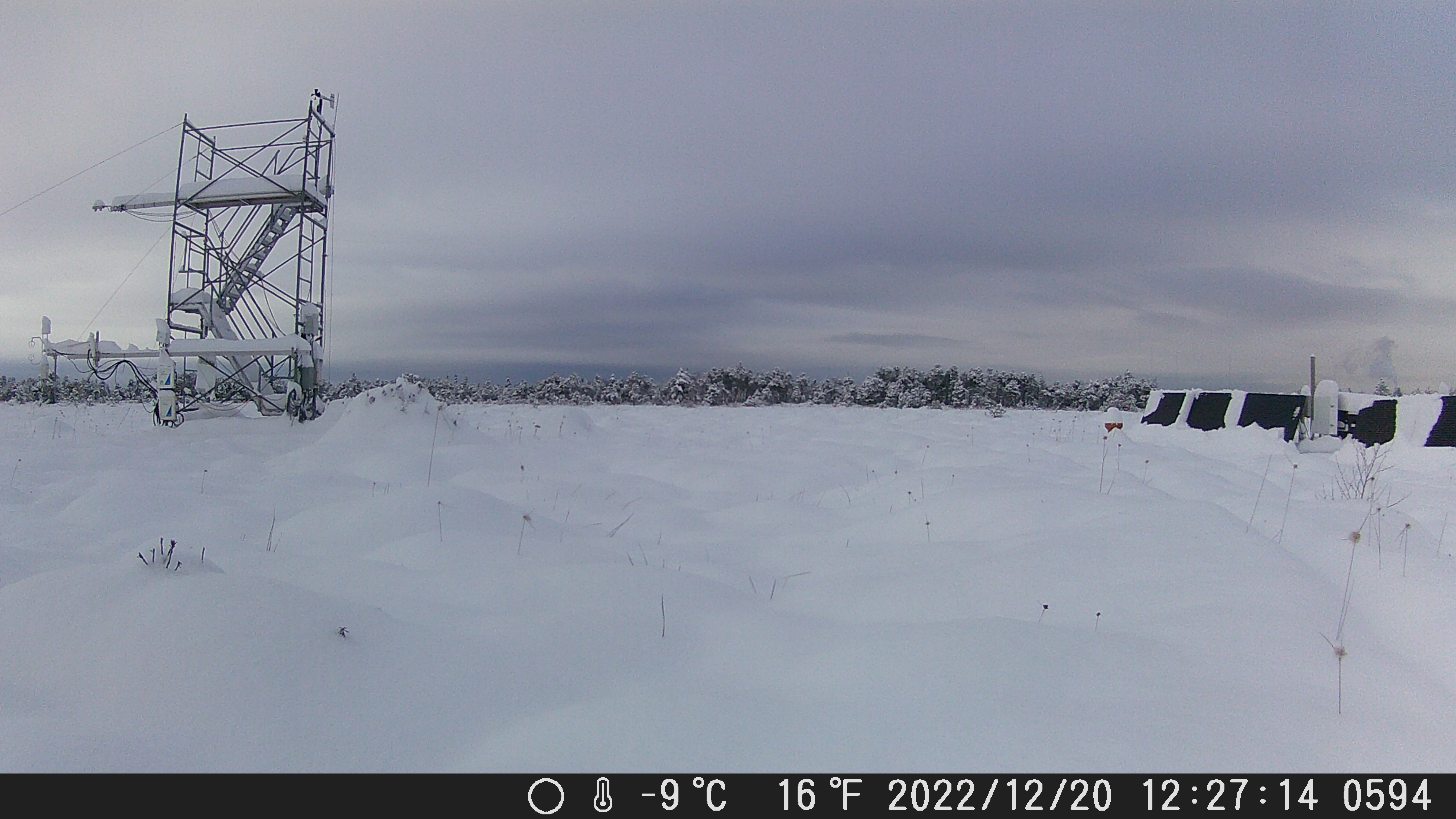
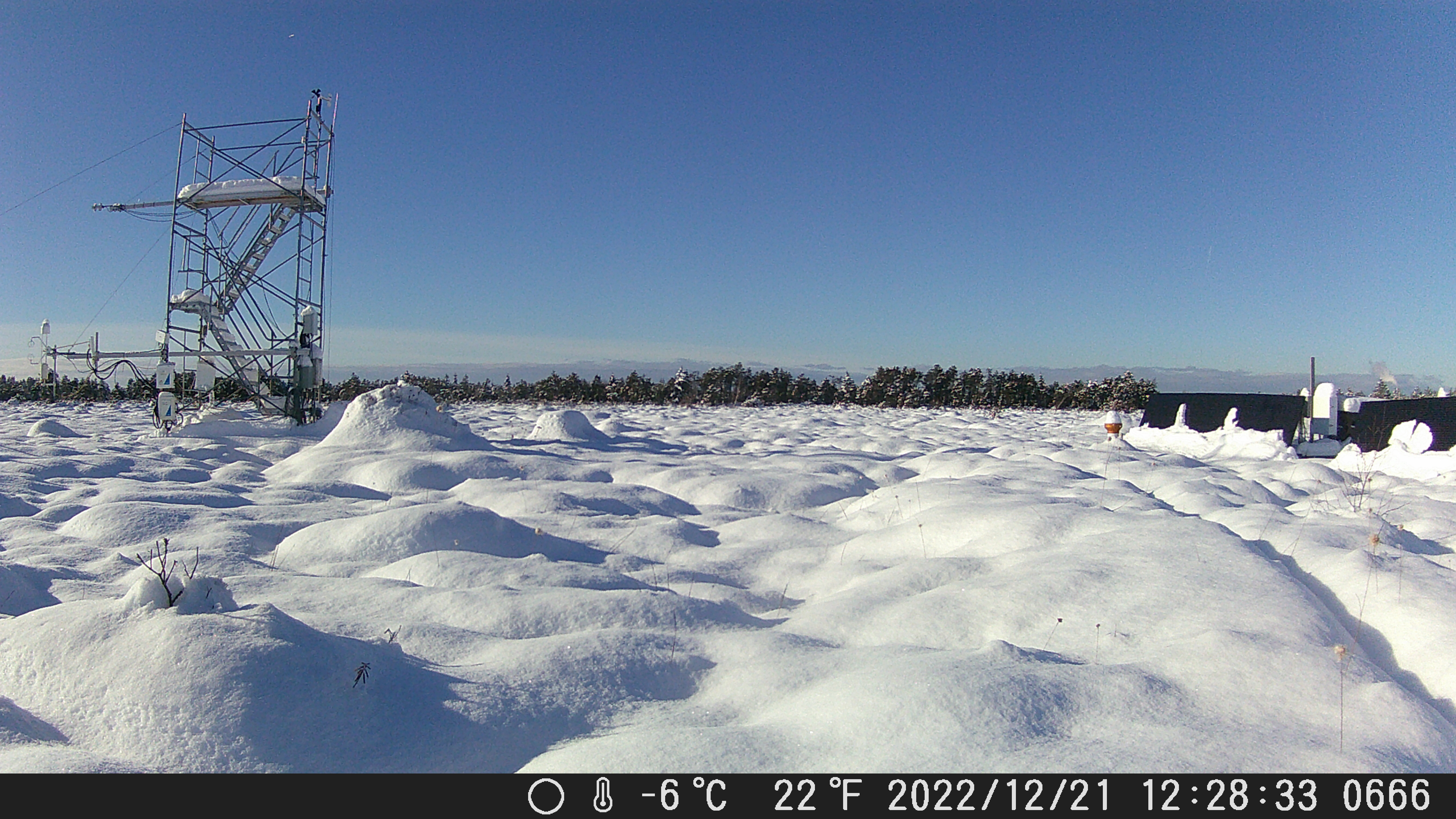
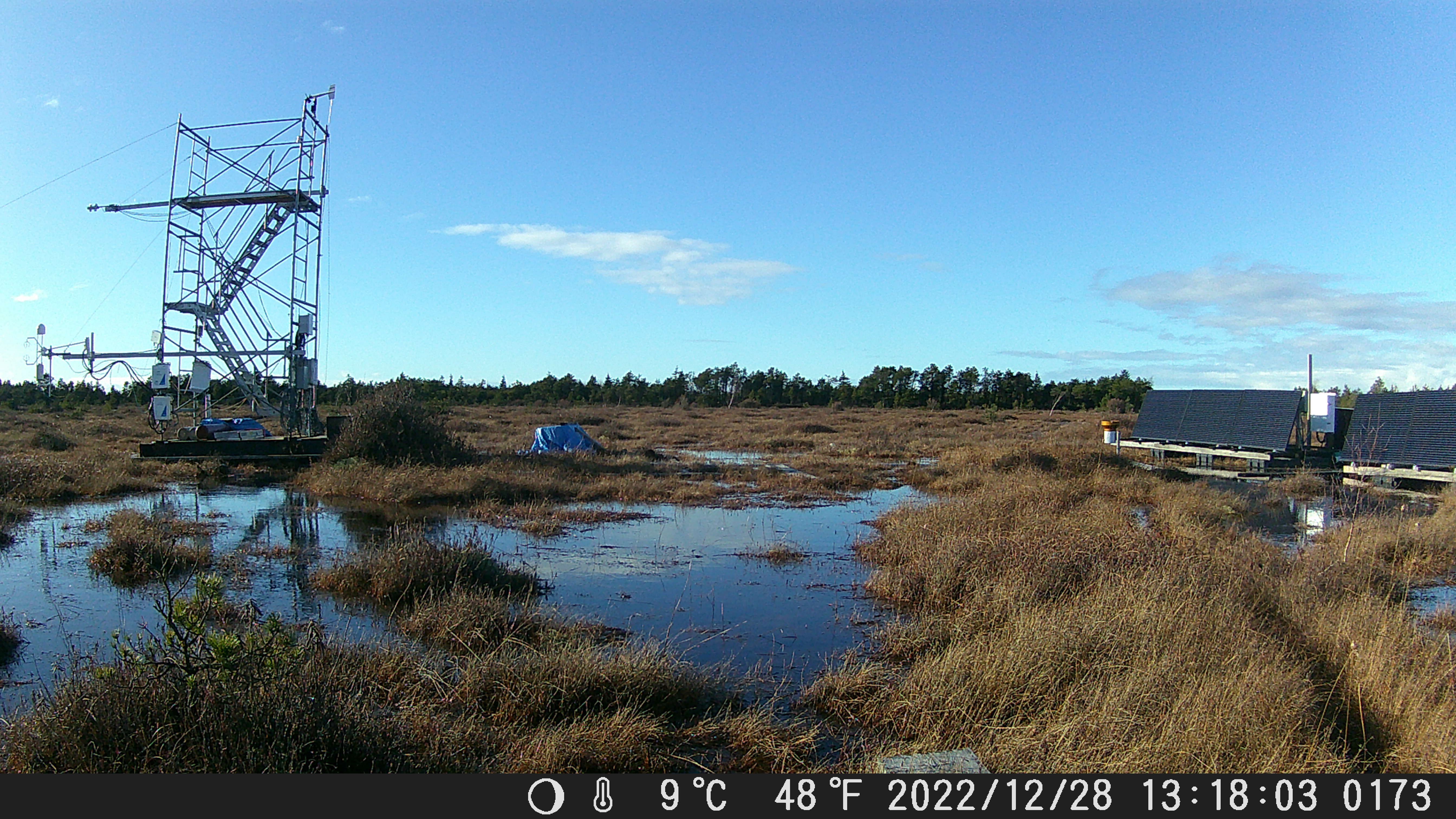
The following questions involve an appreciation of the interaction between separate components of the radiation budgets of sites. Both involve changes in surface radiative properties leading to changes in the budget. Figure 5 shows photos from the Burns Bog Station on four days in late December 2022 which each have different weather conditions. Figure 6 shows the the radiation fluxes that were observed at the site over this time period and Figure 7 shows air temperatures and relative humidity over this time period.

Figure 6: Radiation data from the Burns Bog Flux Station over the winter solstice.

Figure 7: Temperature and humidity data from the Burns Bog Flux Station, late December, 2022.

Question 9 [2.5 points]

Using the data in Figure 6 calculate albedo for timestamps that most closely correspond to each of the time each photo shown in Figure 5 was taken. How do these to values compare to one another? What explains any differences? Do any of these albedo values look suspicions? if so, which day(s) and why?

Answer:

Winter$Albedo <- Winter$SW_OUT_1_1_1/Winter$SW_IN_1_1_1

A <- Winter[Winter$TimeStamp == '2022-12-20 12:30',]
B <- Winter[Winter$TimeStamp == '2022-12-21 12:30',]
C <- Winter[Winter$TimeStamp == '2022-12-27 12:30',]
D <- Winter[Winter$TimeStamp == '2022-12-28 13:30',]

Figure 5 (a): 1.8096537

Figure 5 (b): 0.81352

Figure 5 (c): 0.0661095

Figure 5 (d): 0.1297618

Explanation:

Figure 5 (a) - is suspect because Albedo > 1 (shouldn’t have more outgoing than incoming) - the issue is that the sensor is still covered by the fresh snowfall

The rest are fine - the key differences are that all the snow in Figure 5 (b) has melted in the other images. Snow is a great reflector of \(SW\), hence the high albedo (but <1 so still physically plausible). Figure 5 (c) and Figure 5 (d) are more or less comparable (very low) albedo. Note: this point is not required for full credit(The minor difference would be attributable to the greater fraction of diffuse radiation in Figure 5 (c) compared to more direct radiation in Figure 5 (d)).

Note For TA:

Allow for 1-2% variation incase they pick an adjacent timestep or round their answer

.25 pt per timestep 1.5 pt for the explanation

Question 10 [1 points]

Figure 6 also shows net radiation (\(R_n\)). Notice how the \(R_n\) is negative, during mid-day when Figure 5 (b) was taken. This is somewhat abnormal for the site. However, the data is valid, this not an artifact. Which component of Equation 7 is primarily responsible for the negative value of \(R_n\) at this time step? Can you think of anything that might explain this negative value, which we did not observe during the day when either Figure 5 (c) or Figure 5 (d) were taken? Hint: look at the traces in Figure 7

Answer:

\(LW/downarrow\) is primarily responsible for the negative \(R_n\) - the reason for this can be attributed to atmospheric conditions - \(LW/downarrow\) (and \(LW/uparrow\)) will correspond to temperature - but that alone isnt sufficient to explain it. The sharp contrast in RH (lower RH = drier air) is largely responsible for the dip in \(LW/downarrow\) relative to \(LW/uparrow\). Water vapor absorbs (and therefore re-emits) lots of \(LW\) so all else equal \(LW/downarrow\) will be greater on a day with higher moisture content in the atmosphere. See lecture.

Note For TA:

.25 pt if they only say temperature and ignore RH

Question 11 [0.5 points]

Multiple Choice: select the correct answer(s) from those listed

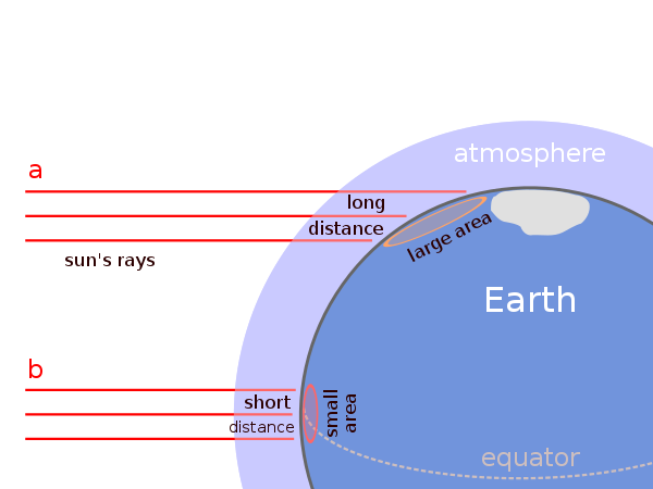
The Burns Bog Station station is a at latitude of 49.5 \(^{\circ}\) and the solar declination on the winter solstice (December 21^st) is -23.5 \(^{\circ}\). The solar constant (\(I_0\)) is approximately 1361 W m^-2. Given this information, the R code shown below Example 2 is using the cosine law of illumination to estimate the effect of beam spreading on incoming solar radiation at the on the winter solstice. Why does the value estimated calculated below not match what was observed at the Burns Bog Site at solar noon on December 21st 2022? Look Figure 5 (b), carefully inspect the \(SW\downarrow\) for that day shown in Figure 6, and reference the lecture materials for help answering this question.

A. Reflection of the solar beam due to cloud cover

B. Attenuation of the solar beam due to Rayleigh scattering in the atmosphere

C. Attenuation of the solar beam due to absorption by Ozone (O₃) in the upper atmosphere

D. Reflection of the solar beam due to snow cover on the ground

Example 2

Solar_Constant = 1361

Solar_Declination_on_Winter_Solstice = -23.5
Latitude = 49.5

# Zenith (at solar noon) is the latitude minus the solar declination
Zenith = Latitude - Solar_Declination_on_Winter_Solstice

# The Cosine Law of Illumination!
# The R "cos()" function requires us to convert the units of the input to be in Radians **Not Degrees**
Zenith_Radias = Zenith*(pi/180)

Irradiance = Solar_Constant * cos(Zenith_Radias) 

# This function formats a text (string) output the "%s" values are replaced with the variable(s) listed after the string
Output <- sprintf('Irradiance on Dec. 21st at %s degrees latitude is %s W m-2 at the top of the atmosphere.', Latitude, round(Irradiance,digits=2))

# This function prints us a cleanly formatted output
writeLines(Output)

Irradiance on Dec. 21st at 49.5 degrees latitude is 397.92 W m-2 at the top of the atmosphere.

Answer:

B & C - Rayleigh scattering will send some shorter wavelength light back to space before it reaches the ground & ozone will absorb a lot of short wave length UV radiation before it reaches the ground.

Not A - there isn’t cloud cover on this day. See Figure 5 (b) & Figure 6.

Not D - the ground/snow is below the pyranometer, so its not an issue. The snow that was on the sensor the day before Figure 5 (a) had melted by Figure 5 (b)

Note For TA:

.25 pt if they only say temperature and ignore RH