| Symbol | Name | Definition |
|---|---|---|
| \(z\) | Vertical position | Relative to Earth’s surface (height or depth) unless otherwise specified |
| ELR | Environmental Lapse Rate | Observed change in air temperature with height |
| DALR | Dry Adiabatic Lapse Rate | -0.01 \(K m^{-1}\) |
| SALR | Saturated Adiabatic Lapse Rate | The rate is variable as a function of \(T\) and \(P\) but we can assume a constant rate of -0.005 \(K m^{-1}\) to get a reasonable approximation |
Lab 4: Vertical Structure of the Atmosphere
This assignment is worth 14.5 points.
Objectives
- Understand the concept related to the vertical structure of the atmosphere, in particular, how temperature changes with height
- Understand the different types of lapse rates
- Environmental lapse rate (ELR)
- Dry adiabatic lapse rate (DALR)
- Saturated adiabatic lapse rate (SALR)
- Understand and concept of static stability and distinguish between different types of stability within a particular air layer
1 Overview
Weather Balloons
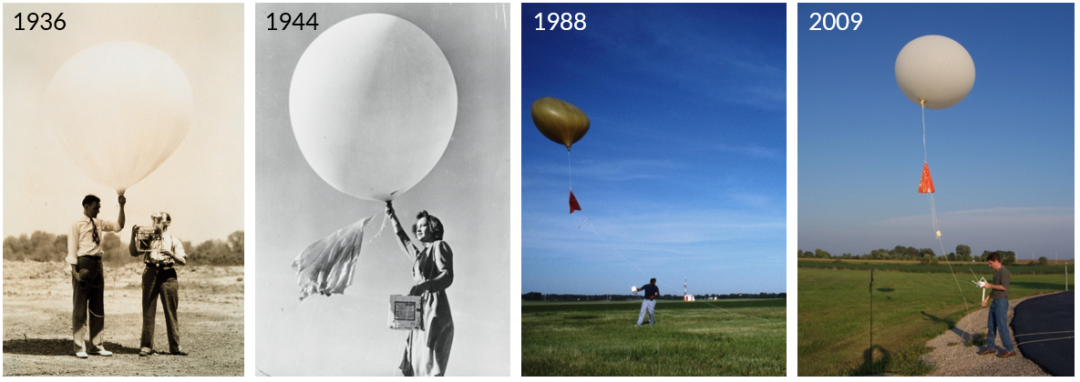
Our understanding of the vertical structure of Earth’s atmosphere has been informed by over a century of weather balloon launches Figure 1. Modern balloons carry sensors to measure temperature, humidity, and air pressure along with a radiosonde which transmits data back to a station on the ground. The balloons record data as they ascend through the atmosphere, giving us a profile of temperature, humidity, and air pressure. Some balloons are also tracked by GPS, which allows wind speed and direction to be calculated as well. Eventually, the balloon pops and it’s transmitter returns to earth via a parachute. Modern balloons regularly reach heights exceeding 30,000 meters above sea level (m.a.s.l); for reference, commercial aircraft fly between 9,000 and 13,000 m.a.s.l
Figure 2 shows a web map weather balloon stations that are part the Integrated Global Radiosonde Archive network. Take a moment to look around the map; note the spatial distribution of stations across Earth’s surface. These data are an important component of weather forecasts as they give us information the current state of the upper atmosphere. They are also used to help validate satellite data products, and historical balloon records are use to train global climate models. Balloon launches at most stations are conducted twice daily at 0:00 UTC and 12:00 UTC. Launch times are kept consistent across the globe by using (UTC time)[https://en.wikipedia.org/wiki/Coordinated_Universal_Time] instead of the local time. This is important for standardizing observations so they can be included in global climate models. If you ever need to convert between UTC time and local time, you can use this tool to help.
Atmospheric Profiles
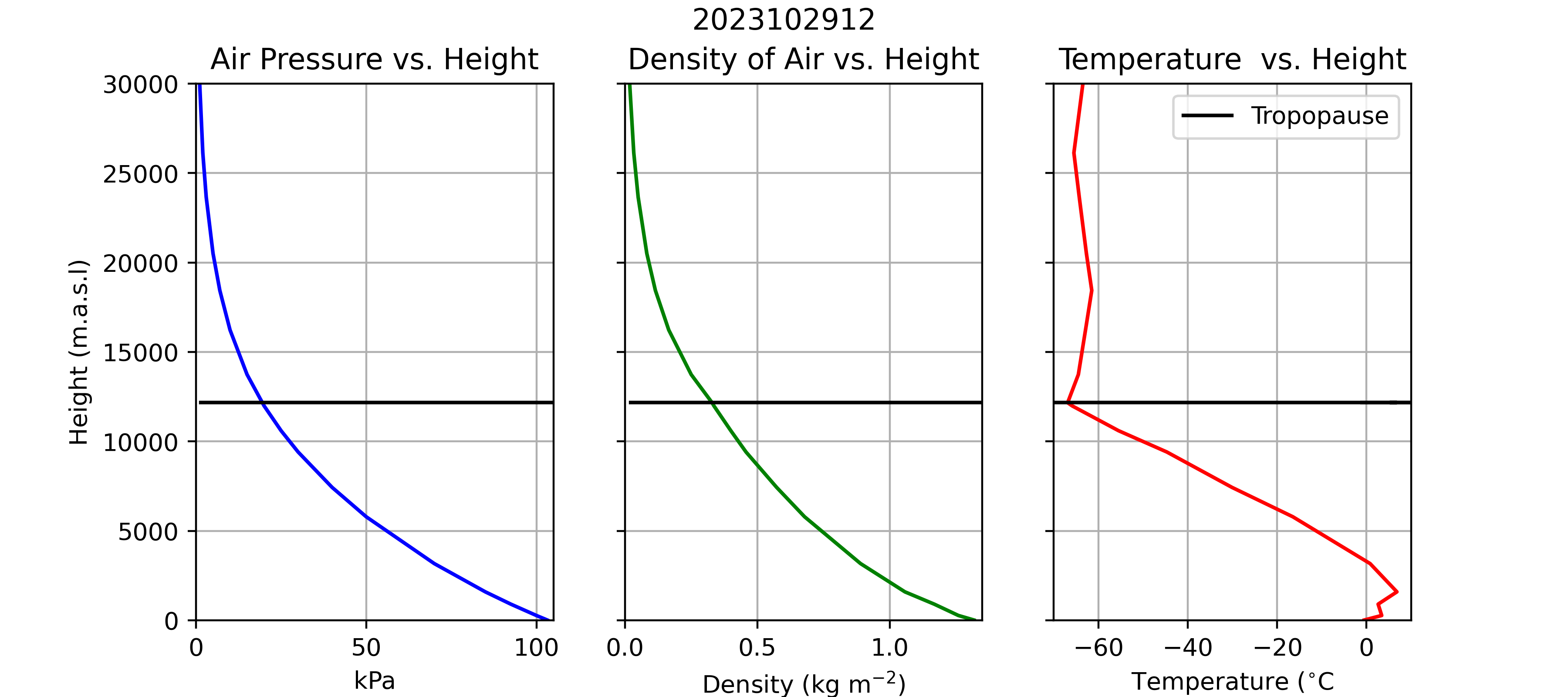
The atmosphere is a compressible gas; i.e., air is compressed by the weight (pressure) of the air above it. Therefore, density (\(\rho\)) and air pressure (\(P\)) decrease with increasing height above the sea level (Figure 3). Note how \(P\) decreases steadily with height, from just over 100 kPa at sea level to less than 10 kPa at 20,000 meters above sea level (m.a.s.l). Air pressure always decreases with height, because air pressure is a function of the weight of air above a measurement location. As you move upwards through the atmosphere, the weight of the air above you decreases, so there is less pressure (compressional force) exerted by the remaining air above you and the density of the air decrease. Near Earth’s surface, the decrease is approximately linear (\(\approx\) -0.012 kPa m-1), but the rate of change decrease at higher elevations.
The relationship between pressure and density is given by the Ideal Gas Law Equation 1. Recall the notation from Lab 3: pressure (\(P\)), volume (\(V\)), temperature (\(T\)), and the amount of the gas (\(n\)) in moles; with \(R\) being the ideal gas constant (see Table 1). The amount in moles of a given gas (or mixture of gasses) can be defined as \(n = \frac{m}{M}\), where \(m\) is the mass of the substance (in kg or g) and \(M\) is the Molar mass (in kg mol-1 or g mol-1) respectively.
\[ PV=nRT \tag{1}\]
You may have noticed this phenomena if you’ve ever been to the top of a tall mountain. Since the atmosphere is less dense on top of a tall mountain, there is less oxygen available with each, and your body has to breathe more heavily to compensate. You probably also noticed that it was cooler atop the mountain. Looking at Equation 1, we can see that a decrease in \(P\) can also lead to a decrease in \(T\). However, \(T\) profiles in the atmosphere aren’t strictly a function of height, as you can see in Figure 3, there are other factors at play, particularly near the surface and above the tropopause.
Questions
Question 1 [1 points]
Looking at Figure 2, what parts of the world (countries/regions) have the most comprehensive weather balloon records? Consider both the density of current observations and the length of historical records in your answer.
Answer:
- India and the United States both have good spatial coverage with many stations having long periods of record (e.g., >90 years).
- China, Russia, and some parts of Europe have good spatial coverage, with many stations having moderate length records (e.g., >50 years)
- Indonesia & Malaysia also have good spatial coverage, but only mostly shorter records (e.g., <50 years)
Notes for TA
- May use regions instead of explicitly naming countries (eg. South Asia instead of India etc.)
- But must mention India & US (or an equivalent region name) for full credit
- If they don’t explicitly mention the other points but offer a thoughtful response or discuss other areas, they can still get full credit.
Question 2 [0.25 points]
Multiple Choice: select the correct answer(s) from those listed
What local time and date would a balloon launch in Port Hardy, BC that occurs at 00:00 UTC November 25th, 2023 correspond to?
- A 5:00 PM November 25th, 2023
- B 4:00 PM November 25th, 2023
- C 4:00 PM November 24th, 2023
- D 4:00 AM November 25th, 2023
C - 4:00 PM November 24th, 2023
Question 3 [1 points]
How does air pressure vary as a function of height relative to sea level and why?
We’re looking for a summary of this explanation
Question 4 [0.75 points]
The dead sea is a salt lake between Jordan, Palestine, and Israel. It has an average surface elevation of 403.5 m below sea level, making it’s shores the lowest land area on Earth’s surface. All else equal, how would you you expect air pressure at the dead sea to compare to air pressure at locations at sea level in the region?
Half credit if they say \(P\) will be lower than that at sea level. Full credit if they calculate the approximate relative difference:
dP_dH = -0.012 #kPa/m
Elevation = -403.5 #m

Relative_Pressure_Difference = Elevation*dP_dH
\(P\) would be \(\approx\) 4.842 kPa higher than that at seas level
2 Lapse Rates
As a consequence of the ideal gas law, when an air parcel is lifted upwards though the atmosphere, its temperate will decrease in correspondence with the decrease in air pressure. Conversely, when a parcel of air sinks its temperature will increase in correspondence with the increase in pressure. This phenomena is known as an adiabatic process: where temperature of a substance changes without the addition/subtraction of energy. When thinking about adiabatic processes, we assume a parcel does not mix with the environment. In reality, this assumption is never perfectly met, but it applies well enough when dealing with large parcels of air.
Adiabatic Processes
The rate at which the parcel will cool depends on whether or not it is saturated. Why? Because the amount of water the atmosphere can hold is a function of temperature. In order for a parcel to cool below its dewpoint water vapor must condense, and the process of condensation releases heat to the surrounding environment.
The dry adiabatic lapse rate (DALR) applies when a parcel of air is not saturated, and has a constant with a value of -0.01 K m-1. The DALR dictates the rate of cooling if a parcel is being lifted upwards or the rate of warming for a parcel that is descending.
The saturated adiabatic lapse rate (SALR) applies once a parcel of air reaches saturation. A saturated parcel still cools as it rises but condensation also occurs which releases latent heat and counteracts some of the cooling. It important to note that the SALR only applies to cooling air, when air warms it will always do so at the DALR, because as soon as the air begins to warm, it will no longer be saturated.
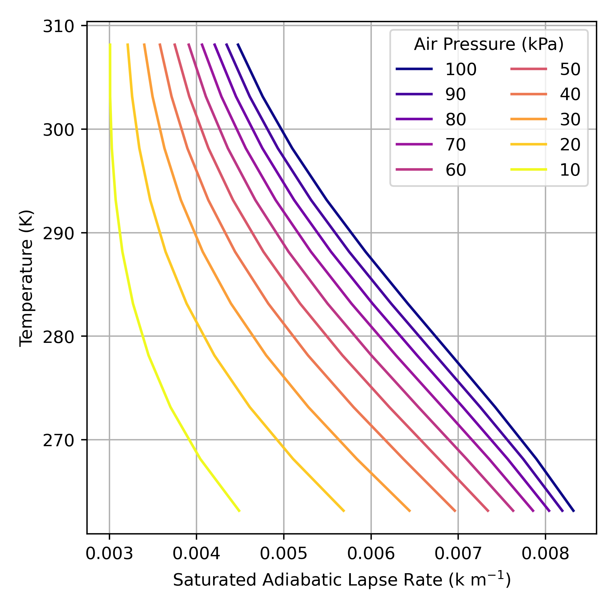
The actual value of the SALR is non-linear function of \(T\) and \(P\); it is shown for selected values of \(T\) and \(P\) in Figure 4. Calculating the exact value of the SALR is complex because:
- \(T\) varies as a function of \(P\)
- The latent heat released by condensation varies as a function of \(T\)
- The amount of water that must condense for a parcel to cool also varies as a function of \(T\)
While the SALR is not constant you will can see from Figure 4 that changes in \(T\) and \(P\) have opposing effects on the SALR. A decrease in \(T\) increases the SALR while a decrease in \(P\) will decrease SALR. Given this, we can assume a constant SALR of -0.005 K m-1 to perform reasonably accurate approximations.
Environmental Laps Rate
The observed rate of change of \(T\) with height at a given location know the environmental lapse rate (ELR). We can determine the ELR directly from weather balloon data or estimate it from weather forecast models. The ELR rate varies drastically between locations, heights, and times. It can be calculated between any two heights in a balloon profile using Equation 2. A positive ELR indicates that \(T\) increases with height whereas a negative ELR indicates \(T\) it decreases with height.
\[ ELR = \frac{T_{z_2}-T_{z_1}}{z_2-z_1} \tag{2}\]
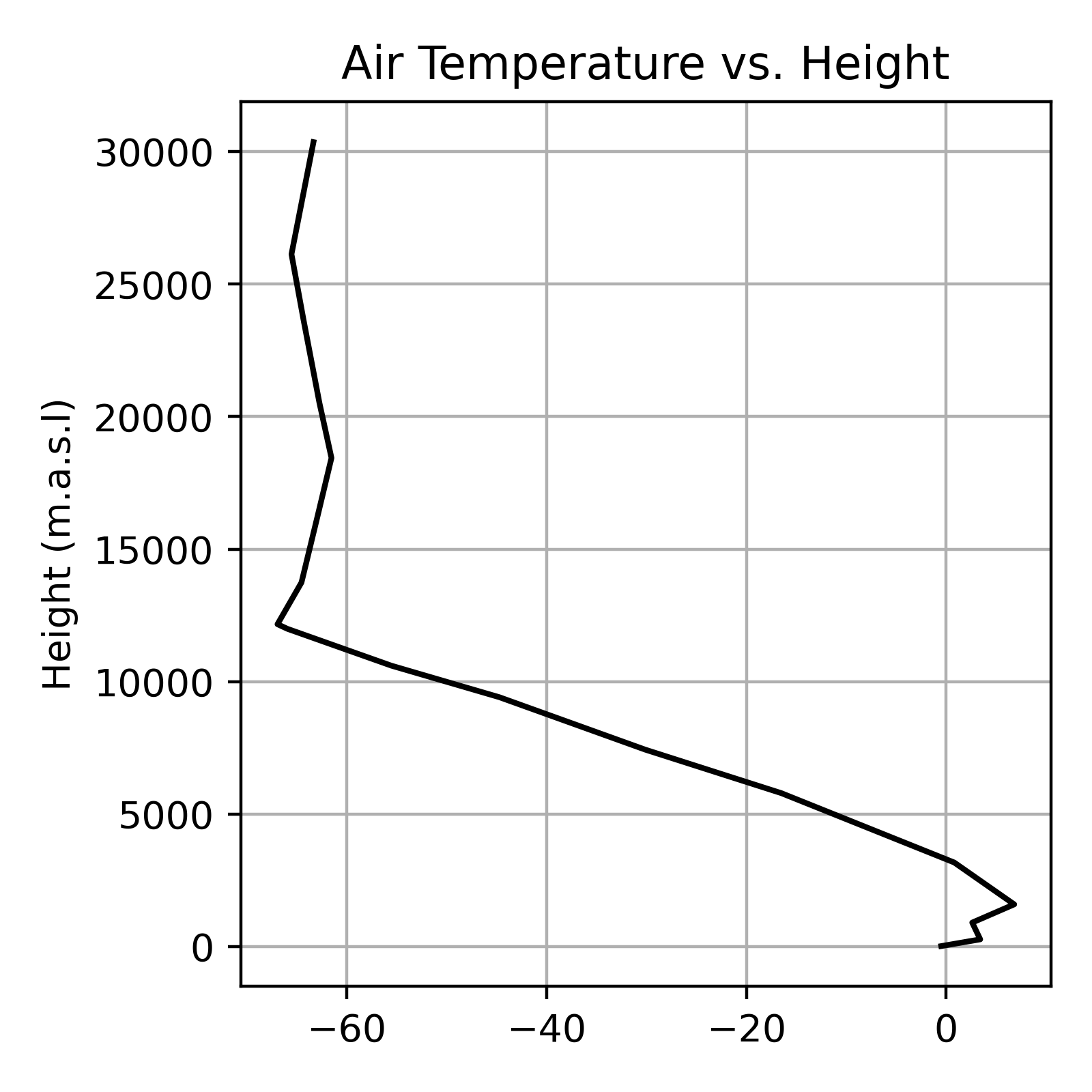
Figure 5 and Table 2 show an example atmospheric temperature profile. Note how \(T\) tends to decrease with height but does do not always decrease as a function of height. A temperature inversion occurs when warmer air is found above cooler air. In Figure 5, there is a strong temperature inversions present near the surface. This is a common occurrence on calm clear nights when radiative cooling (\(LW\) emissions) at the Earth’s surface cause air near the surface to cool more than air above the surface. You will also note there is a temperature inversion around 12,500 m.a.s.l. This is known as the tropopause; the boundary between the troposphere and the stratosphere (we’ll discuss this distinction in lecture).
| Height (m.a.s.l) | ELR K/m | |
|---|---|---|
| 1 | 17 | NA |
| 2 | 271 | 0.0154 |
| 3 | 904 | -0.0013 |
| 4 | 1592 | 0.0061 |
| 5 | 3172 | -0.0038 |
| 6 | 5790 | -0.0066 |
| 7 | 7430 | -0.0083 |
| 8 | 9410 | -0.0074 |
| 9 | 10600 | -0.0091 |
| 10 | 11990 | -0.0075 |
| 11 | 12165 | -0.0057 |
| 12 | 13740 | 0.0015 |
| 13 | 16230 | 0.0006 |
| 14 | 18440 | 0.0006 |
| 15 | 20510 | -0.0006 |
| 16 | 23660 | -0.0005 |
Lifting Condensation Level
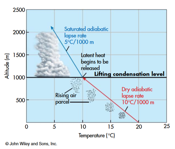
When a parcel of air is lifted, it will cool at the DALR, until it becomes saturated. Once saturated, condensation will begin to occur, the parcel will cool at the SALR, and clouds will start to form. This height where the transition occurs is know as the Lifting Condensation Level (LCL), which is the level where \(T=T_d\). The LCL corresponds the to the bottom of a cloud layer. The LCL (in m.a.s.l) for a parcel at \(z_1\) will be a function of the parcel’s dewpoint depression; the difference between the parcel’s air temperature (\(T_{z_1}\)) and its dewpoint (\(T_{dz_1}\)):
\[ LCL = \frac{T_{dz_1}-T_{z_1}}{DALR}+z_1 \tag{3}\]
The numerator in Equation 3 will tell us who much a parcel needs to cool in order to reach it’s dewpoint, the denominator tells us how many meters the parcel needs to rise from it’s current position, and subtracting \(z_1\) puts in standard terms (m.a.s.l). Recall: the parcel will not mix well with its surroundings so its starting properties (e.g., water vapor content) will be preserved. So while \(T\) will decrease adiabatically as a parcel is lifted, \(T_d\) will remain unchanged.
- In Figure 6, a parcel at the surface (\(z_1\) = 0 m.a.s.l) has \(T = 20^{\circ}C\) and \(T_d = 10^{\circ}C\), the parcel must cool by 10 \(^{\circ}C\) for \(T=T_d\) and condensation will begin. With the DALR = -0.01 K m-1; \(LCL = \frac{10 ^{\circ}C - 20 ^{\circ}C}{-0.01 K m^{-1}} + 0 m.a.s.l- = 1000 m.a.s.l.\).
- Note Lapse rates are given in K, we don’t need to convert \(T\) and \(T_d\) to K first, because 1 \(^{\circ}C\) = 1 K. Any time you calculate the difference between two temperatures in \(^{\circ}C\) the resulting value is also the difference in K.
Adiabatic Process Equation
A generalize formula for approximating the temperature of a parcel (\(T_p\)) that moves from one level (\(z_1\)) to another (\(z_2\)), is given in Equation 4. If a parcel is rising (\(z_1 < z-2\)), it will cool at the DALR until reaching the LCL and then cool at the SALR. Note that above the LCL, the parcel’s dewpoint (\(T_{dp}\)) will decrease in lockstep with \(T_p\). If a parcel is descending (\(z_1 > z_2\)) it will warm at the DALR over the entire descent while the \(T_{dp}\) will not change.
\[ T_p(z_2) = \begin{cases} T_p(z_1) + min((LCL-z_1),(z_2-z_1)) * DALR + max(z_2-LCL,0) * SALR \ , \text{if} z_2>z_1 \\ T_p(z_1) + (z_2-z_1) * DALR \ , \text{if} z_1>z_2 \end{cases} \tag{4}\]
Questions
Question 5 [1.5 points]
Why is the SALR is lower than than the DALR?
When a parcel rises, it will cool adiabatically. But for a saturated parcel to cool, condensation must occur. Laten heat released by condensation counteracts some (but not all) of the adiabatic cooling.
Question 6 [2 points]
An air parcel at \(z_1\) = 100 m.a.s.l with \(T\) = 30 \(^{\circ}\) C and \(T_d\) = 21 \(^{\circ}\) C is displaced upwards to \(z_2\) = 1500 m.a.s.l. What will the parcel’s \(T\) and \(T_d\) be at when it reaches \(z_2\)? Will clouds form during the ascent, and if so, at what height will they begin to form?
APE <- function(T1,TD1,Z1,Z2){
  DALR = -0.01
  SALR = -0.005
  LCL = (TD1-T1)/DALR+Z1
  if(Z1 > Z2){
    T2 = T1 + (Z2-Z1)*DALR
  } else {
    T2 = T1 + min((LCL-Z1),(Z2-Z1))*DALR + max(Z2-LCL,0)*SALR
  }
  if(T2<TD1){
    TD2 = T2
  }
  else {
    TD2 = TD1
  }
  return(c(LCL,T2,TD2))
}


out = APE(T_z1,T_dz1,z1,z2)
Clouds will begin forming at the LCL (1000 m.a.s.l). At \(z_2\); \(T\) = 18.5 C and \(T_d\) 18.5 C
Question 7 [1 points]
An air parcel at \(z_1\) = 2000 m.a.s.l with \(T\) = 7 \(^{\circ}\) C and \(T_d\) = 5 \(^{\circ}\) C is displaced downwards to \(z_2\) = 100 m.a.s.l. What will the parcel’s \(T\) and \(T_d\) be at when it reaches \(z_2\)?
out = APE(T_z1,T_dz1,z1,z2)At \(z_2\); \(T\) = 26 C and \(T_d\) 5 C
3 Atmospheric Stability
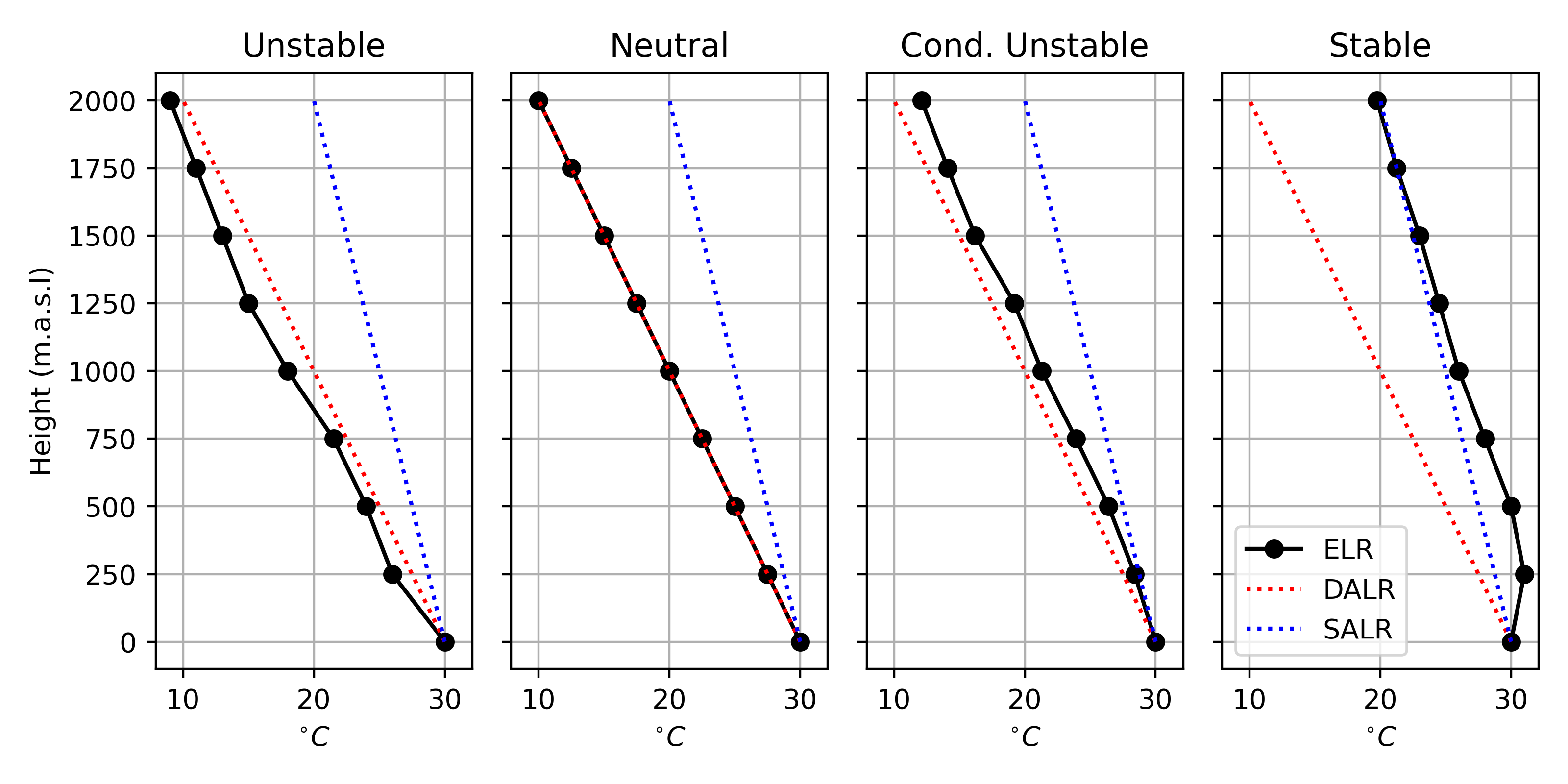
You’ve probably heard that “hot air rises”. All else equal, when air is warmer than it’s surrounding environment, it has a tendency to expand; following Equation 1 \(V\) will increase, making the air less dense than its surroundings. You can assess the stability of the atmosphere by comparing the ELR to the DALR and the SALR. Four different stability conditions are discussed bellow with examples show in Figure 8
Stable
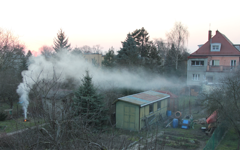
When the ELR > SALR there will be no tendency for a parcel to rise or sink after it is displaced. If an air parcel is displaced upwards, it will become cooler and more dense than the surrounding air and tend to sink back to its original location. If displaced below, it will find itself warmer and tend to rise back up to its original location. In a stable layer, vertical movements are suppressed. In very stable conditions, such as those present when there is a temperature inversion, smoke and other air pollutants accumulate and often cause respiratory problems.
Unstable
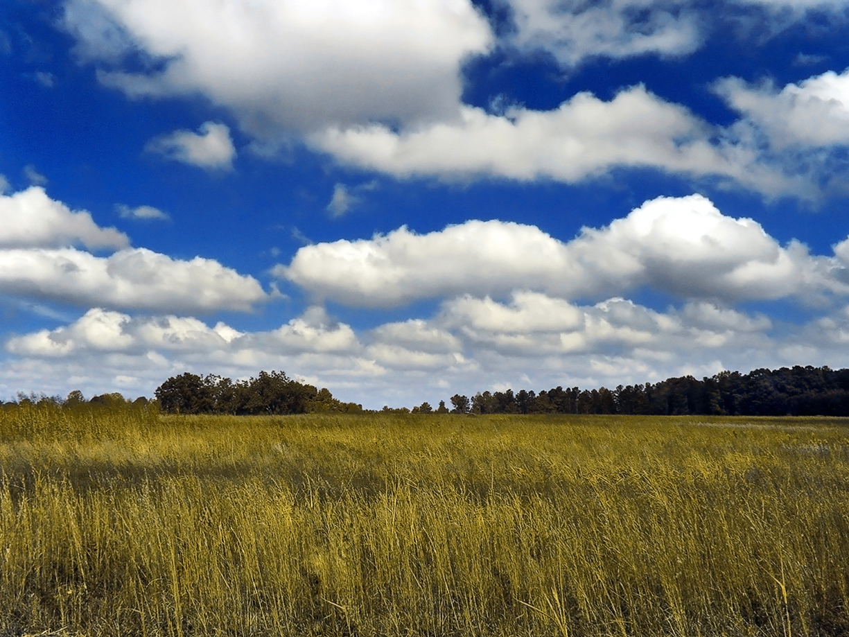
When the ELR < DALR any upward displacement will result in a continuous rise of an parcel. As it rises it will cool following the DALR (or SALR once it cools to its dewpoint). The parcel will become warmer and less dense than the surrounding air, giving it buoyancy. Conversely, if the air parcel is displaced downwards, it will become cooler and more dense than the surrounding air at the same height, and it will tend to continue sinking. This upward and downward movement of air is know as convection. These conditions promote the development of cumulus clouds (the light fluffy looking ones) and can often result in thunderstorms.
Neutral Stability
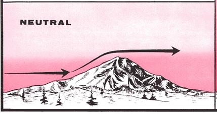
When ELR = DALR, vertical motion isn’t enhanced or suppressed for dry air. This typically occurs in the absence of significant heating or cooling (e.g., heavy cloud cover) or during periods of high winds. If a parcel is lifted by some external force e.g., flowing over a mountain as shown in Figure 7, it will tend to remain at this new elevation.
Conditionally Unstable
This is a special case when the SALR \(\geq\) ELR \(\geq\) DALR, conditions are said to be conditionally unstable. A dry parcel of air that is displaced will act as a stable parcel and sink back to its original position. However, if a saturated parcel is displaced then it will act as an unstable parcel and convicting will occur. By definition, neutral conditions are also conditionally unstable.
Questions
Question 8 [2 points]
Looking at Table 2, give the atmospheric stability for each layer (unstable, conditionally unstable, or stable). You can find a copy of the data from the table here. Note: you can assume a constant SALR of -0.005 \(K\ m^{-1}\). Given this, how would you characterize the stability of the atmosphere at this location on this day? If there were a forest fire in the area, what would happen to the smoke from the fire?
The atmosphere is stable near the surface, there is a region of conditional instability in the middle elevations, but no unstable conditions anywhere. Given the temperature inversion, smoke from the fire would not mix with the air above, it would accumulate near the surface.
| Height (m.a.s.l) | ELR K/m | Stability | |
|---|---|---|---|
| 1 | 17 | – | – |
| 2 | 271 | 0.0154 | Stable |
| 3 | 904 | -0.0013 | Stable |
| 4 | 1592 | 0.0061 | Stable |
| 5 | 3172 | -0.0038 | Stable |
| 6 | 5790 | -0.0066 | Conditionally Unstable |
| 7 | 7430 | -0.0083 | Conditionally Unstable |
| 8 | 9410 | -0.0074 | Conditionally Unstable |
| 9 | 10600 | -0.0091 | Conditionally Unstable |
| 10 | 11990 | -0.0075 | Conditionally Unstable |
| 11 | 12165 | -0.0057 | Conditionally Unstable |
| 12 | 13740 | 0.0015 | Stable |
| 13 | 16230 | 0.0006 | Stable |
| 14 | 18440 | 0.0006 | Stable |
| 15 | 20510 | -0.0006 | Stable |
| 16 | 23660 | -0.0005 | Stable |
4 Observations
In this portion of the lab, you will work on interpreting some weather balloon data yourself. Each student has been randomly assigned two datasets, representing balloon launches from stations somewhere in Canada. One balloon launch occurred sometime at 12:00 UTC during winter 2022, and the other occurred at 00:00 UTC in summer 2022. You can find the station code along with the dates of the winter and summer balloon launches you are responsible for here. You can download the weather balloon data here. The data are in .zip file format, you must extract the data to find your data files. Open the IGRA_CA_Data folder after extracting it, you will see a set of folders that correspond to the station codes of assorted Canadian weather balloon station. Each folder contains a set of .csv files that correspond to dates/times of balloon launches. The file names are in YYYYMMDDHH (Year-Month-Day-Hour) format. Find the files that correspond to the Winter and Summer dates you were assigned.
Questions
Question 9 [5 points]
What is the name of the balloon station you’ve been assigned? Where is it located and what is it the station’s elevation? Note List your student number here to make it easier for your TA to mark your answer.
For both balloon profiles you have been assigned:
- Make a plot showing the \(T\) and \(T_d\) change with height. You can sketch this by hand or make a graph using a software package like excel. Include the date/time of the balloon launch along with the station name and elevation in the title of each graph.
- Calculate the ELR using the temperature readings for each height interval and determine the atmospheric stability for each interval. You can list these as a table.
0.5 pt for correct answers
These are going to vary by student and by summer/winter
- 1 pts for a. for both winter and summer; 1.25 pts each for b. for both winter and summer